
Show me the POCUS
Knobs and More
In this chapter we present settings on the ultrasound machine that help you optimize your view. This is known as Knobology, the knowledge of how to achieve the correct machine adjustments for the best image quality and to maximize the potential of US equipment functions. The reader is invited to review the physics notes for a refresher on some of concepts explained here.

Unfocused beam. The ultrasound probe generates a beam that starts along its diameter. This beam generated is parallel from its origin, travels and ultimately diverges as it penetrates through tissue. The interface between that near field parallel beam and the beam that diverges is the focal point. Axial resolution is best seen in the near field and the maximal point of resolution is at the focal POINT.
Focused beam. The beam is now forced to focus on selected depth and enters tissue at a converging angle towards the narrowest diameter, the focal ZONE. This causes the resolution to be highest at this depth at the cost of worse resolution at a depth further from the focal zone. The focal zone is the part of the US beam where its diameter is focused and narrowest. The beam then increases again after the focal zone. The focal zone is determined by the transducer diameter and frequency. This best axial resolution occurs when you select the focal length to be at the at the structure of interest.
Focus
Focused vs non-focused. On the left a Focused ultrasound beam with narrowest diameter located at the focal zone (dark circle). The near field in red is also known as the Fresnal Zone while the far field in dashed magenta is the Far field (or Fraunhofer). Notice the divergence seen on the far field. On the right, an unfocused ultrasound beam parallel to the probe diameter. Notice the lower far field divergence with this probe.
The length of the near field (Fn) is proportional to the transducer footprint squared and inversely related to the wavelength of the probe. A higher frequency probe with a large footprint will have the furthest near field. On the opposite terms a low frequency probe with a small footprint has the lowest near field. This implies that if you want the best resolution for a given structure you want to select a probe with the biggest footprint with the highest resolution.
Let's compare different focused distances:
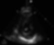
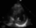
Focused depth set at the anteroseptal wall (see the x's in the image representing the selected focused depth). The posterior wall appears blurry in comparison
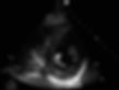
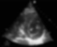
Focused depth set to the posterior wall. Image resolution of this wall has improved as we have better definition of the borders.
Depth
This setting controls the vertical depth of the field of view. Increasing the depth allows deeper tissue interrogation at a cost. This increased depth increases the scan time since the machine will need to wait longer to hear returning echoes from deeper structures; both transmit and receiving time are increased. This in turn increases the time per frame which decreases the frame rate. Using a lower frequency probe may allow us to see deeper structures but this also makes the shallow structures to have loss in resolution. An increased scanning time also causes a lower maximum detectable velocity that can be measured on Color Flow Doppler. Set depth to the target structure for optimal depth.
Let's compare:
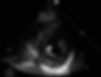
Setting optimal depth so we can visualize the walls of the ventricles that fill up the whole sector.
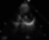
Structure appears too far and borders are not clearly seen.
Sector Scan Size
The imaging sector is the area that is interrogated and displayed on the ultrasound machine. Think of it as the area that you are interrogating and that is most commonly manipulated when using curvilinear probes. The size of the scan can be manipulated using the button on the display (on image). The position of that field of view can also be adjusted. Decreasing the scan size is the same as using less scanning lines per image and thus improves the frame rate. Using this function on Color Flow Doppler allows us to measure speeds more accurately.
Let's compare:

Narrow scan sector

Wide scan sector
Gain
Gain adjusts the displayed amplitude of the returning signals and increasing it causes an increase of all returning signals. Think of this as using a megaphone on the signals. Operationally for optimal settings look at areas in the sector that should not have any physical structures such as vessels or cavities. The gain should be increased until some returning signals are seen and then decreased.
Let's compare:
Optimal gain set so that blood appears black. This can be automatically set by the system by using the iSCAN button.
The gain has been increased on these clips. Blood now has a hypoechoic and not the typical anechoic appearance.

TGC has been increased on the middle distance of the sector causing an overgain of the structures on that 'band' of ultrasound.

iSCAN has been turned on to automatically adjust gain. Alternatively reducing the middle 'band' of TGC has the same effect.
Time Gain Compensation
Here we adjust the gain of the returning signals based on the depth of interest. We can expect that at deeper structures this feature might be turned in a ramped up configuration.
Let's compare:
Frequency
This setting changes the resolution or penetration of the scan. We can toggle between the different frequency capabilities of the probe or its bandwidth. We can choose between having higher frequencies (RES), general (GEN) and penetration (PEN) modes.
On these clips we compare the extremes:

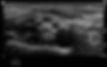
Resolution frequency has been selected on this clip. We can have a better appreciation of the brachial plexus with this supraclavicular view.
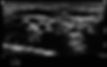
Penetration frequency has been selected on this clip. The same supraclavicular view but this time the brachial plexus is ill defined.
Dynamic Range
The dynamic range refers to the amplitude (and not frequency) of the returning signals. Specifically it is the range (minimal to maximal) of amplitudes that the system is capable of displaying. Adjusting the dynamic range will not change the amplitudes of the returned signal, only of how that returned signal is displayed. Increasing the dynamic range allows you to see very low and very high amplitudes on the display and thus a wide range of grayscale. Borders appear grainy or blurry. A low dynamic range allows you to see higher low amplitude signals and lower higher amplitude signals. Think of this as cutting a segment of all possible returning signals. What we now see is a display with sharper, more defined edges. If this range if further decreased to 0 we see only black and white pixels displayed.
In the following images only dynamic range has been altered and extremes are showed for comparison:
Low dynamic range creates images that have less of 'shades' of gray on the range of different combinations of white and black.

Very high dynamic range on the other hand creates images that appear blurry since there are no absolute white or black.
Harmonics
We allow the probe to transmit in one frequency but it receives signals in multiples of the transmitted frequencies. Improved structure resolution results from harmonic scanning. Harmonic imaging is especially useful in patients where the endocardial border is difficult to visualize. However it may make some other images appear with worse resolution.
Lets compare:
Optimal view of the brachial plexus with the supraclavicular view. Harmonics are not ON.
Harmonics have been turned ON. The returning signals cause significant noise distortion on this image.
References
1. Zander D, Hüske S, Hoffmann B, et al. Ultrasound Image Optimization ("Knobology"): B-Mode. Ultrasound Int Open. 2020;6(1):E14-E24. doi:10.1055/a-1223-1134